Example: Methanol to Olefins (MTO) Model
Here, we illustrate kinetic estimation and reactor optimization for the methanol to olefins reaction. If this is your first attempt at building a project in REX, we suggest that you look at the Ethylene Oxide to Ethylene Glycol example first and then return to this example.
The methanol to olefins system has been studied for several decades and a discussion of mechanisms is available in Park et al. [1]. In this example, we choose a simplified mechanism and the main focus is to illustrate the estimation and optimization of this system in REX. For learning purposes, you may build this project entirely yourself by following the steps below. The experimental data and initial parameter estimates are provided in the MTO_Example.xls file located in the Optience Corporation\REX Suite\REX Examples folder of your installation directory. However, we have also provided the completed project, so you may import the MTO_Example.rex file stored in the same directory and refer to it as you are building the project.
This document shows the steps in building this project without going into the details of the REX features in each node. If at any stage you need help on some node, just press F1 key and a help screen will guide you on the information for the node.
Kinetic Estimation
The methanol to olefins system has been studied for several decades and a discussion of mechanisms is available in Park et al. [1]. In this example, we choose a simplified mechanism and the main focus is to illustrate the estimation and optimization of this system in REX. For learning purposes, you may build this project entirely yourself by following the steps below. The experimental data and initial parameter estimates are provided in the MTO_Example.xls file located in the Optience Corporation\REX Suite\REX Examples folder of your installation directory. However, we have also provided the completed project, so you may import the MTO_Example.rex file stored in the same directory and refer to it as you are building the project.
This document shows the steps in building this project without going into the details of the REX features in each node. If at any stage you need help on some node, just press F1 key and a help screen will guide you on the information for the node.
First, we will estimate the kinetics of the MTO reaction from Experimental data. We will enter the reaction mechanism, kinetics and experimental data to generate the kinetic model for this system. This kinetic model will be then used to optimize the reactor to maximize reaction performance.
The simplified MTO reaction model contains two main group of reactions:
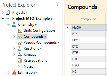
We then add the compounds and reactions written above. Nitrogen is used as a diluent in the Experiments, so N2 must also be added as a compound.
Please enter the compounds as shown below:
In the Compounds → Formula node, you may add the atomic formulae for each compound. This step is optional and is needed only to calculate the atom balance errors for the experiments, as will be shown later in this example.
After entering the compounds, please enter the reactions shown above in the Reactions node. In this project, we also need to monitor and use some additional variables, such as the total carbon content of C3 and C4 olefins. In order to do that, we create pseudo-compounds, which can be defined in the PseudoCompounds node:
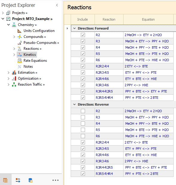
Next, we specify the reaction kinetics in the Kinetics node.
As the methylations are all irreversible, only the forward direction is included. For scissions that are reversible, both directions must be included.
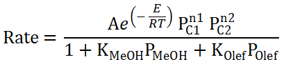
We will use a simplified kinetics model, in which all reactions have order of compounds same as their molecularity (stoichiometry coefficients). Additionally, this reaction is catalysed by solid catalyst and therefore modeled using the Langmuir Hinshelwood (LHHW) models that considers inhibition due to surface adsorption. The LHHW Site for all reactions contains two terms, one for MeOH and another term for the POlef pseudocompound that represents the partial pressure of all olefins.
Thus all reactions have their rate basically described as:
Here, the compound orders n1 and n2 are set to the molecularity of the compounds C1 and C2 in the reaction and we can conveniently build this by going to Kinetics → Parameters node and executing the Initialize Order action. With this action, all reactions will automatically have their compound orders set to their stoichiometric coefficients. R2R3-R5 for instance, will have order 1 for ETY and PPY in the forward direction and order 1 for PTE in the reverse direction.
You may now paste the initial values for the Preexponentials and Activation Energies from the first sheet of the excel file MTO_Example.xls, located in Optience Corporation\REX Suite\REX Examples folder.
Next, we define the LHHW Site that we name AcidSite in the LHHW Sites tab of the same node.
Its constant value is 1, and it has two terms, both of them with initial preexponential values of 5 and energy values of 0:
In the Estimation node, all reactions and directions are selected as Estimate; the LHHW site is also selected to be estimated.
Now the bounds for preexponentials are opened by using the Initialize Mass action Bounds → By Percent of Current action in Estimation → Parameters node. Please choose the Lower and Upper Limit to be 10% and 1000% respectively. The same action should also be done for the LHHW Site preexponentials.
For the activation energy bounds, you may copy them from the second sheet of the MTO_Example.xls file. For most reactions, the forward direction will have lower and upper bounds of 0 and 80 kJ/mol, while the reverse direction will have 0 and 180 kJ/mol as bounds. The activation energy bounds for R2 and R2R2-R4 reactions will be fixed to their initial values. As you will note later in the experimental data with Ethylene feed, dimerization does not occur so this reaction R2R2-R4 is set to have zero rate. The Energy terms for LHHW Site Terms are not estimated and so their bounds are closed at zero.
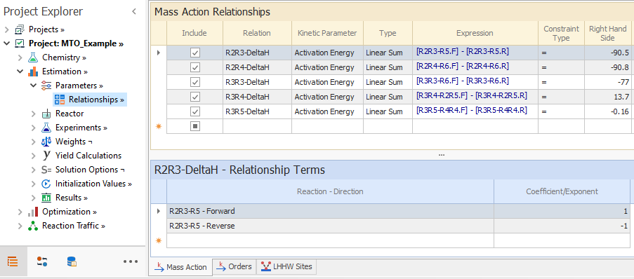
During estimation, we would like to enforce thermodynamic constraints on the activation energies of the scission reactions so that the difference between forward and reverse activation energy values is equal to the heat of reaction. These constraints are added in the Estimation → Parameters → Relationships node, where the Right Hand Side values are the heat of reaction:
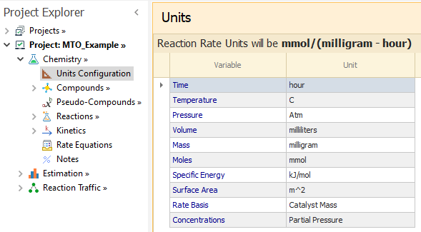
Next, we set the conditions in the Reactor node to be a Single Gas PFR reactor with no recycle. Pressure and Temperature are constant. The pressure is specified in the experimental data, so the Flow is selected as Float for Pressure Control.
The first step here is to enter the experimental sets in the Experiments node. The list of sets is shown in the MTO_Example.xls file - in column B of the Experimental_Design sheet.
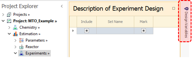
We may also add optional information about the experiment design here. In order to do that, we move the mouse to the Design Variables pane:
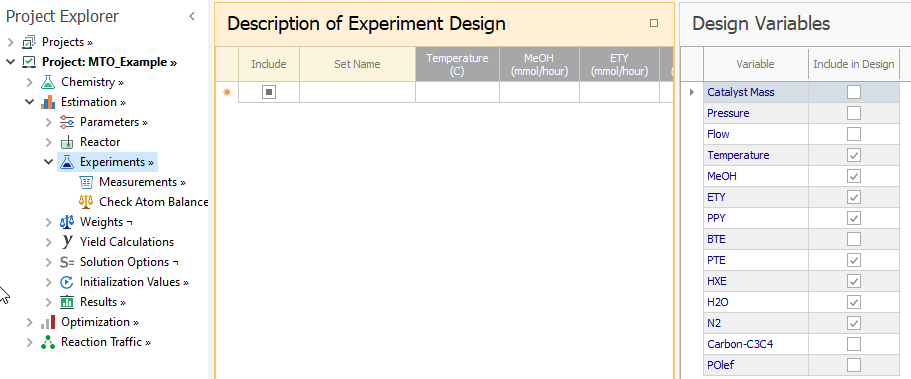
We then select the following variables which are part of the experiment design:
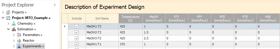
You may now copy the information on the selected design variables from the Experimental_Design sheet for each set:
These values (with the grey header columns) are optional and are meant for the sole purpose of documenting the experiment design.
The actual data for the experimental sets used in the REX calculations is entered next.
In the Experiments → Measurements node, we select all the variables except the pseudocompounds. The child nodes of this node allow you to enter data for each experimental set. For each set, you must have the exact number of datapoints as indicated in the Experimental_Data excel sheet. You can manually add datapoints, or execute the Add Datapoint action to add several datapoints for each set.
Following that, the data in the Experimental_Data sheet is to be entered in the Experiments → Measurements → Sets node. One way to copy data for all sets in a single step is by merging all sets by executing the Merge Sets action in the parent Measurements node. This puts all the experimental data sets in one grid for easy data transfer from Excel.
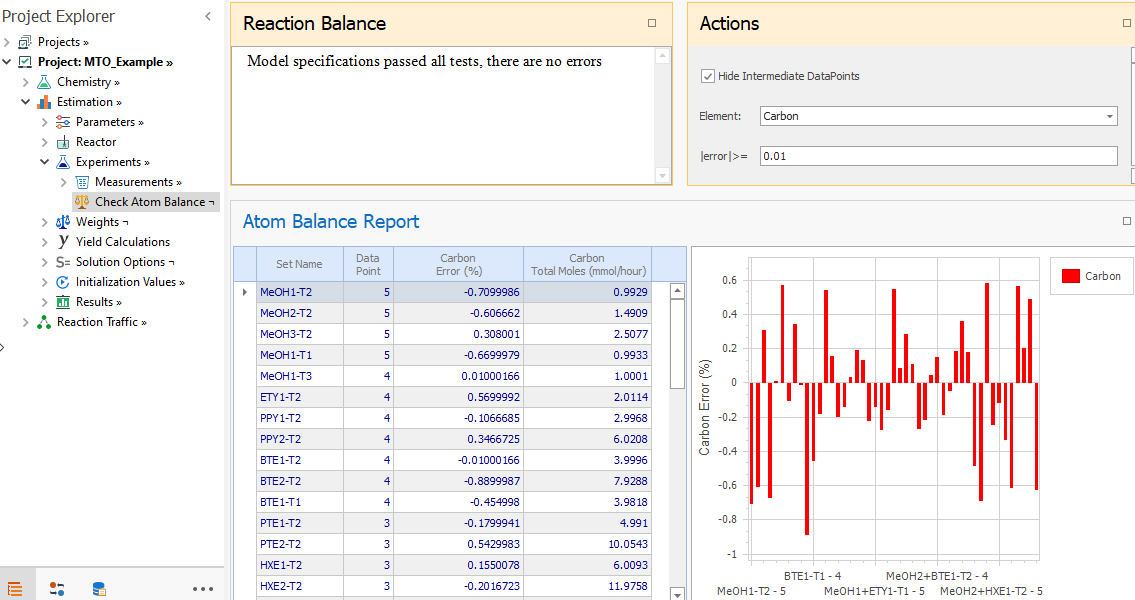
If you have loaded the atom counts for each compound in the Compounds → Formula node, you can check if the reaction stoichiometry was correctly entered by going to the Check Atom Balance node. Also, the carbon error for the experimental sets can be obtained there:
You may review all the data loaded so far by importing the file MTO_Example.rex from Optience Corporation\REX Suite\REX Examples folder and find any differences between your project and the imported project, by using the Compare Projects tool.
In order to estimate the model parameters, you must select the measurements to be reconciled with the data.
This is done in the Weights node, where we include all olefins and MeOH. Weighting factors should be generated with the Hybrid method.
Now you may proceed with the estimation task. By default, in the Solution Options node, the option for Kinetics Parameters is selected as Estimate; thus the parameters of estimated reactions and LHHW Sites are to be found between their bounds by minimizing the weighted Least Square error (LSQ) for all reconciled compounds.
After running the project, you may review the all the results in the Results tree. Also the reaction network and carbon traffic for instance, can be visualized in Reaction Traffic node.
If the estimation was successful, please upload the solution values from the Results → Parameters node into the initial values in the Chemistry → Kinetics → Parameters node and Estimation → Parameters node. This way, the project can be used later for simulation or optimization with the optimally estimated parameters.
To do this, execute the Initialize from Results → All action from either the Estimation or the Initialization Values nodes.
In the Results → Parameters node you can see that preexponential for both forward and reverse directions of R2R2-R4 reaction are zero. Thus, this closed reaction can be eliminated from the model by un-including it from either the Chemistry → Reactions or Chemistry → Kinetics nodes.
The simplified MTO reaction model contains two main group of reactions:
- Methylations: Irreversible reactions where Methanol (MeOH) addition produces higher olefins:
-
R2: 2*MeOH ⇒ ETY + 2*H2O Ethylene formation
R3: MeOH + ETY ⇒ PPY + H2O Propylene formation
R4: MeOH + PPY ⇒ BTE + H2O Butene formation
R5: MeOH + BTE ⇒ PTE + H2O Pentene formation
R6: MeOH + PTE ⇒ HXE + H2O Hexene formation
- Oligomerization/Scissions: Reversible reactions where Olefins react by merging or splitting :
-
R2R2-R4: 2*ETY ⇔ BTE
R2R3-R5: ETY + PPY ⇔ PTE
R2R4-R6: ETY + BTE ⇔ HXE
R3R3-R6: 2*PPY ⇔ HXE
R3R4-R2R5: PPY + BTE ⇔ ETY + PTE
R3R5-R4R4: PPY + PTE ⇔ 2*BTE
|
|---|
We then add the compounds and reactions written above. Nitrogen is used as a diluent in the Experiments, so N2 must also be added as a compound.
Please enter the compounds as shown below:
|
|---|
In the Compounds → Formula node, you may add the atomic formulae for each compound. This step is optional and is needed only to calculate the atom balance errors for the experiments, as will be shown later in this example.
After entering the compounds, please enter the reactions shown above in the Reactions node. In this project, we also need to monitor and use some additional variables, such as the total carbon content of C3 and C4 olefins. In order to do that, we create pseudo-compounds, which can be defined in the PseudoCompounds node:
- Carbon-C3C4 = 3*PPY + 4*BTE
Since this is a linear combination of moles, we select this variable as Conserved, which allows REX to treat this like a compound and report the moles of this Carbon-C3C4 variable in the model results. If Conserved is not selected, this variable is only calculated in the concentration units.
- POlef = ETY + PPY + BTE + PTE + HXE
This variable represents the total concentration of Olefins, which is to be used later in the kinetics model.
Next, we specify the reaction kinetics in the Kinetics node.
As the methylations are all irreversible, only the forward direction is included. For scissions that are reversible, both directions must be included.
|
|---|
We will use a simplified kinetics model, in which all reactions have order of compounds same as their molecularity (stoichiometry coefficients). Additionally, this reaction is catalysed by solid catalyst and therefore modeled using the Langmuir Hinshelwood (LHHW) models that considers inhibition due to surface adsorption. The LHHW Site for all reactions contains two terms, one for MeOH and another term for the POlef pseudocompound that represents the partial pressure of all olefins.
Thus all reactions have their rate basically described as:
|
|---|
Here, the compound orders n1 and n2 are set to the molecularity of the compounds C1 and C2 in the reaction and we can conveniently build this by going to Kinetics → Parameters node and executing the Initialize Order action. With this action, all reactions will automatically have their compound orders set to their stoichiometric coefficients. R2R3-R5 for instance, will have order 1 for ETY and PPY in the forward direction and order 1 for PTE in the reverse direction.
You may now paste the initial values for the Preexponentials and Activation Energies from the first sheet of the excel file MTO_Example.xls, located in Optience Corporation\REX Suite\REX Examples folder.
Next, we define the LHHW Site that we name AcidSite in the LHHW Sites tab of the same node.
Its constant value is 1, and it has two terms, both of them with initial preexponential values of 5 and energy values of 0:
- Term1: It has order 1 respect to MeOH.
- Term2: It has order 1 respect to pseudocompound POlef, that represents the partial pressure of all olefins.
In the Estimation node, all reactions and directions are selected as Estimate; the LHHW site is also selected to be estimated.
Now the bounds for preexponentials are opened by using the Initialize Mass action Bounds → By Percent of Current action in Estimation → Parameters node. Please choose the Lower and Upper Limit to be 10% and 1000% respectively. The same action should also be done for the LHHW Site preexponentials.
For the activation energy bounds, you may copy them from the second sheet of the MTO_Example.xls file. For most reactions, the forward direction will have lower and upper bounds of 0 and 80 kJ/mol, while the reverse direction will have 0 and 180 kJ/mol as bounds. The activation energy bounds for R2 and R2R2-R4 reactions will be fixed to their initial values. As you will note later in the experimental data with Ethylene feed, dimerization does not occur so this reaction R2R2-R4 is set to have zero rate. The Energy terms for LHHW Site Terms are not estimated and so their bounds are closed at zero.
During estimation, we would like to enforce thermodynamic constraints on the activation energies of the scission reactions so that the difference between forward and reverse activation energy values is equal to the heat of reaction. These constraints are added in the Estimation → Parameters → Relationships node, where the Right Hand Side values are the heat of reaction:
|
|---|
Next, we set the conditions in the Reactor node to be a Single Gas PFR reactor with no recycle. Pressure and Temperature are constant. The pressure is specified in the experimental data, so the Flow is selected as Float for Pressure Control.
The first step here is to enter the experimental sets in the Experiments node. The list of sets is shown in the MTO_Example.xls file - in column B of the Experimental_Design sheet.
We may also add optional information about the experiment design here. In order to do that, we move the mouse to the Design Variables pane:
|
|---|
We then select the following variables which are part of the experiment design:
|
|---|
You may now copy the information on the selected design variables from the Experimental_Design sheet for each set:
|
|---|
These values (with the grey header columns) are optional and are meant for the sole purpose of documenting the experiment design.
The actual data for the experimental sets used in the REX calculations is entered next.
In the Experiments → Measurements node, we select all the variables except the pseudocompounds. The child nodes of this node allow you to enter data for each experimental set. For each set, you must have the exact number of datapoints as indicated in the Experimental_Data excel sheet. You can manually add datapoints, or execute the Add Datapoint action to add several datapoints for each set.
Following that, the data in the Experimental_Data sheet is to be entered in the Experiments → Measurements → Sets node. One way to copy data for all sets in a single step is by merging all sets by executing the Merge Sets action in the parent Measurements node. This puts all the experimental data sets in one grid for easy data transfer from Excel.
If you have loaded the atom counts for each compound in the Compounds → Formula node, you can check if the reaction stoichiometry was correctly entered by going to the Check Atom Balance node. Also, the carbon error for the experimental sets can be obtained there:
|
|---|
You may review all the data loaded so far by importing the file MTO_Example.rex from Optience Corporation\REX Suite\REX Examples folder and find any differences between your project and the imported project, by using the Compare Projects tool.
In order to estimate the model parameters, you must select the measurements to be reconciled with the data.
This is done in the Weights node, where we include all olefins and MeOH. Weighting factors should be generated with the Hybrid method.
Now you may proceed with the estimation task. By default, in the Solution Options node, the option for Kinetics Parameters is selected as Estimate; thus the parameters of estimated reactions and LHHW Sites are to be found between their bounds by minimizing the weighted Least Square error (LSQ) for all reconciled compounds.
After running the project, you may review the all the results in the Results tree. Also the reaction network and carbon traffic for instance, can be visualized in Reaction Traffic node.
If the estimation was successful, please upload the solution values from the Results → Parameters node into the initial values in the Chemistry → Kinetics → Parameters node and Estimation → Parameters node. This way, the project can be used later for simulation or optimization with the optimally estimated parameters.
To do this, execute the Initialize from Results → All action from either the Estimation or the Initialization Values nodes.
In the Results → Parameters node you can see that preexponential for both forward and reverse directions of R2R2-R4 reaction are zero. Thus, this closed reaction can be eliminated from the model by un-including it from either the Chemistry → Reactions or Chemistry → Kinetics nodes.
Mode Optimization
When the kinetics of a reaction are known, either from the results of an estimation project or from the literature, we can use the optimization features in REX to improve the reactor performance. We will now show how to maximize the carbon yield of (PPY + BTE) with respect to carbon from the main reactant (MeOH).
If you wish to build the optimization project yourself, you can start from your estimation project and switch to Optimization mode by executing the Mode → Change to Optimization action. Following that, you can set the reactor to be the same that defined for estimation mode by executing the Load Reactor Data action in the Optimization → Reactor node. Alternately, you may directly view the completed Optimization setup in the provided MTO_Example.rex file after switching the project to optimization mode.
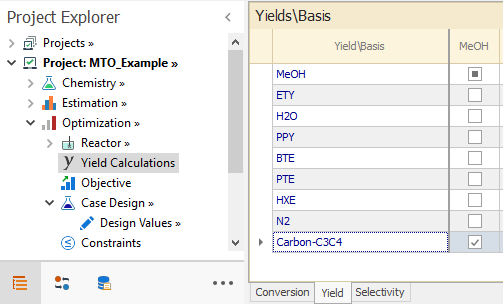
In the Optimization → Yields Calculations node, we define the Yield of pseudocompound = Carbon-C3C4 with respect to MeOH:
The Carbon-C3C4 variable defined in PseudoCompounds node adds the carbon content for Propylene and Butene, while carbon moles for the reactant MeOH just the moles of MeOH.
Other Yields, Conversions or Selectivities can be defined here to be monitored. However, only those that have non-zero weights in the Objective node are considered for the optimization.
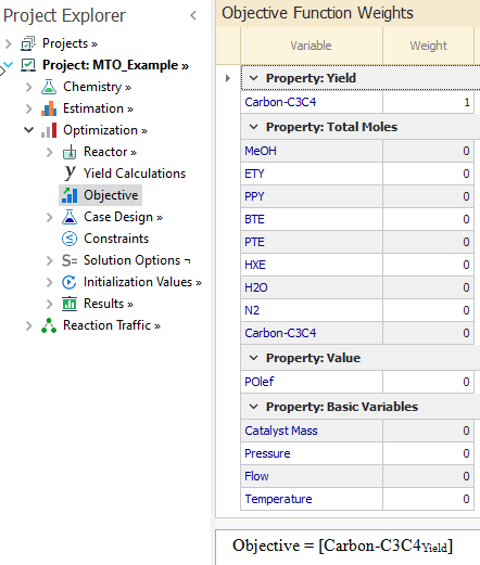
In this example, we want only to maximize the yield of Carbon-C3C4. Thus, a weight of 1 is entered for Carbon-C3C4 and all other variables have zero weights:
You may then define the Case-Opt case in the Case Design node. The Specifications and Initial Charge bounds are provided in the Design_Values sheet of the the excel file MTO_Example.xls.
In this example, the initial charge for all compounds are fixed, while the Catalyst Mass and Temperature have open bounds in order to find their optimal values. Pressure is fixed while the Flow has open bounds to the maintain pressure at its setpoint.
In order to have better accuracy on the variable profiles, please increase the number of finite elements to 20 in the Optimization → Solution Options node.
On running the project, you should obtain the maximum yield value of 70.71%, which is reported in the Results node.
In the Results → Reactor Summary node, we see that the optimal Catalyst Mass is 23.189 mg, while the optimal Temperature value is 417.78 C.
If you were able to get the above solution successfully, please execute the Initialize from Results → All action from either the Optimization or the Initialization Values node. This way, future runs will all have all variables initialized with the solution values from this last run, facilitating faster solver convergence.
Next, we attempt to improve yield further, by allowing the Temperature to have a profile (non-constant) along the reactor.
This is done by enabling Control Profiles in Optimization node. The Control Profiles tree appears, where the Temperature must be selected to be optimized.
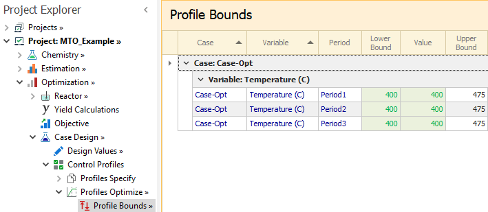
In the Profiles Optimize node, the reactor length is split into three periods of nearly equal length as shown below. For all of them, a linear profile is selected for the Temperature:
Finally, in the Profile Bounds node, Temperature bounds and values are entered for each period:
We see that the yield increases from 70.71% when using constant optimized temperature, to 77.33% now that temperature profile is optimized.
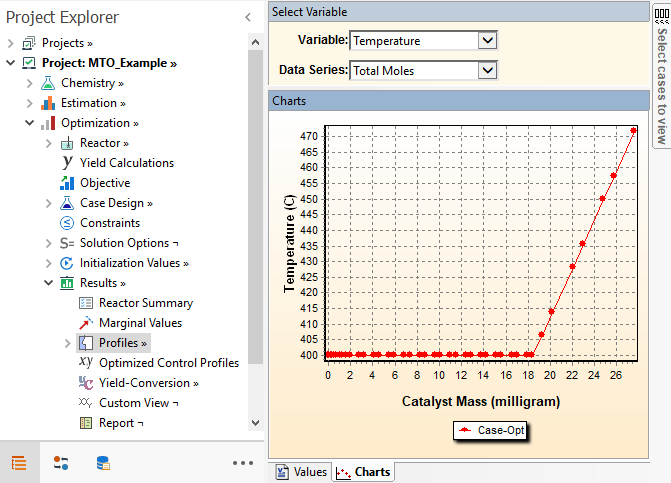
The optimal temperature profiles can be seen in the Results → Profiles node:
The Temperature stays at the lower bound for the first and second period, then goes up in the third period. The reason is that in the beginning, lower temperature promotes the higher olefins (because they have lower activation energy). Once MeOH is depleted, these higher olefins can be split to C3 and C4 by increasing temperature. The reaction R2 that produces Ethylene has the highest activation energy. If we run higher temperature in the beginning, the Ethylene fraction becomes higher and that Ethylene cannot be converted to Butene once the Methanol is exhausted. This is because the R2R2-R4 reaction has zero rate. This optimal profile allows less of the MeOH to be stored as Ethylene in the beginning and once Methanol is depleted, higher temperature promotes the scission of higher olefins to increase C3 (mainly) and C4 olefins. Reactant MeOH decreases from the reactor inlet and becomes negligible close to the reactor outlet:
1. Tae-Yun Park and Gilbert F. Froment, Analysis of Fundamental Reaction Rates in the Methanol-to-Olefins Process on ZSM-5 as a Basis for Reactor Design and Operation, Industrial & Engineering Chemistry Research 2004 43 (3), 682-689
Top of Topic If you wish to build the optimization project yourself, you can start from your estimation project and switch to Optimization mode by executing the Mode → Change to Optimization action. Following that, you can set the reactor to be the same that defined for estimation mode by executing the Load Reactor Data action in the Optimization → Reactor node. Alternately, you may directly view the completed Optimization setup in the provided MTO_Example.rex file after switching the project to optimization mode.
In the Optimization → Yields Calculations node, we define the Yield of pseudocompound = Carbon-C3C4 with respect to MeOH:
|
|---|
The Carbon-C3C4 variable defined in PseudoCompounds node adds the carbon content for Propylene and Butene, while carbon moles for the reactant MeOH just the moles of MeOH.
Other Yields, Conversions or Selectivities can be defined here to be monitored. However, only those that have non-zero weights in the Objective node are considered for the optimization.
In this example, we want only to maximize the yield of Carbon-C3C4. Thus, a weight of 1 is entered for Carbon-C3C4 and all other variables have zero weights:
|
|---|
You may then define the Case-Opt case in the Case Design node. The Specifications and Initial Charge bounds are provided in the Design_Values sheet of the the excel file MTO_Example.xls.
In this example, the initial charge for all compounds are fixed, while the Catalyst Mass and Temperature have open bounds in order to find their optimal values. Pressure is fixed while the Flow has open bounds to the maintain pressure at its setpoint.
In order to have better accuracy on the variable profiles, please increase the number of finite elements to 20 in the Optimization → Solution Options node.
On running the project, you should obtain the maximum yield value of 70.71%, which is reported in the Results node.
In the Results → Reactor Summary node, we see that the optimal Catalyst Mass is 23.189 mg, while the optimal Temperature value is 417.78 C.
If you were able to get the above solution successfully, please execute the Initialize from Results → All action from either the Optimization or the Initialization Values node. This way, future runs will all have all variables initialized with the solution values from this last run, facilitating faster solver convergence.
Next, we attempt to improve yield further, by allowing the Temperature to have a profile (non-constant) along the reactor.
This is done by enabling Control Profiles in Optimization node. The Control Profiles tree appears, where the Temperature must be selected to be optimized.
In the Profiles Optimize node, the reactor length is split into three periods of nearly equal length as shown below. For all of them, a linear profile is selected for the Temperature:

|
|---|
Finally, in the Profile Bounds node, Temperature bounds and values are entered for each period:
|
|---|
We see that the yield increases from 70.71% when using constant optimized temperature, to 77.33% now that temperature profile is optimized.
The optimal temperature profiles can be seen in the Results → Profiles node:
|
|---|
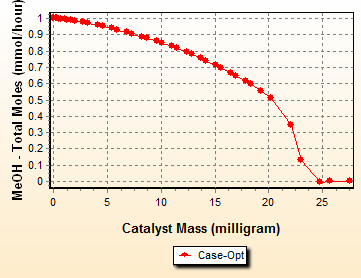
The Temperature stays at the lower bound for the first and second period, then goes up in the third period. The reason is that in the beginning, lower temperature promotes the higher olefins (because they have lower activation energy). Once MeOH is depleted, these higher olefins can be split to C3 and C4 by increasing temperature. The reaction R2 that produces Ethylene has the highest activation energy. If we run higher temperature in the beginning, the Ethylene fraction becomes higher and that Ethylene cannot be converted to Butene once the Methanol is exhausted. This is because the R2R2-R4 reaction has zero rate. This optimal profile allows less of the MeOH to be stored as Ethylene in the beginning and once Methanol is depleted, higher temperature promotes the scission of higher olefins to increase C3 (mainly) and C4 olefins. Reactant MeOH decreases from the reactor inlet and becomes negligible close to the reactor outlet:
|
|---|
1. Tae-Yun Park and Gilbert F. Froment, Analysis of Fundamental Reaction Rates in the Methanol-to-Olefins Process on ZSM-5 as a Basis for Reactor Design and Operation, Industrial & Engineering Chemistry Research 2004 43 (3), 682-689